Class Imbalance and Problem Statement
Class imbalance is a common problem when building classifiers in the machine learning world, and our awesome previously-scraped croc reviews data is unfortunately not so awesome from a class balance standpoint. Soon, we’ll assign binary class labels based on the rating a customer gave with their review where we’ll consider ratings of 2 stars (out of 5) or less to be negative sentiment and the remaining reviews as positive sentiment. As you’ll see in a moment, the vast majority of reviews belong to the positive sentiment class, and I think that’s great!
However, I don’t believe Crocs reached the top of the shoe game by mistake. I’d be willing to bet the creators behind Crocs are more than willing to confront their flaws and improve upon them. Let’s pretend the good people behind Crocs have asked us to build an ML model to effectively classify the rare negative review for their product despite the severe class imbalance. They don’t mind a few misclassifications of the positive reviews here and there but would prefer there aren’t a ton of these instances.
Quick Note on Positive / Negative Lingo
Traditionally, the positive class in a binary labeled dataset is the minority class of most interest / importance, and that will hold true in this project. Apologies for any confusion, but going forward when I reference the positive class, I will be referencing the set of negative sentiment reviews.
- Positive Class (1) - Negative Sentiment Review :(
- Negative Class (0) - Positive Sentiment Review :)
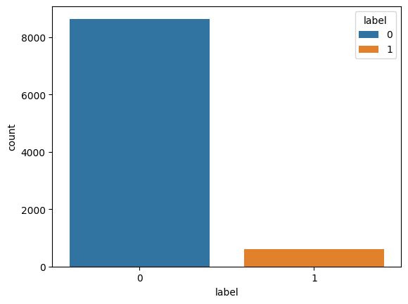
Below is a look at the class imbalance of our data.
import pandas as pd
from collections import Counter
import seaborn as sns

df = pd.read_csv('/content/drive/MyDrive/croc_reviews.csv')
df['label'] = [0 if each > 2 else 1 for each in df['rating']]
sns.countplot(x = df['label'], hue = df['label'])
print("Only", "{:.0%}".format(label_count[1] / (label_count[1] + label_count[0])), "of our data belongs to the positive class.")
Only 6% of our data belongs to the positive class.
Data Clean Up
Before we start addressing the class imbalance issue, let’s clean up the reviews using the text cleaning function we’ve used before.
import re
import string
import nltk
from nltk.corpus import stopwords
from nltk.stem import PorterStemmer

def clean_text(text):
    # Remove punctuation
    text = re.sub(f"[{re.escape(string.punctuation)}]", "", text)

    # Remove numbers
    text = re.sub(r'\d+', '', text)

    # Convert to lowercase
    text = text.lower()

    # Remove stopwords
    nltk.download('stopwords', quiet=True)
    stop_words = set(stopwords.words('english'))

    tokens = nltk.word_tokenize(text)
    tokens = [word for word in tokens if word.lower() not in stop_words]

    # Stemming
    stemmer = PorterStemmer()
    tokens = [stemmer.stem(word) for word in tokens]

    # Join the tokens back into a single string
    cleaned_text = ' '.join(tokens)

    return cleaned_text

df['clean_review'] = [clean_text(text_to_clean) for text_to_clean in df['review']]
df
| review | date | rating | label | clean_review | |
|---|---|---|---|---|---|
| 0 | !!!!!! E X C E L L E N T!!!!!!!!!! | April 7, 2022 | 5.0 | 0 | e x c e l l e n |
| 1 | "They're crocs; people know what crocs are." | April 3, 2021 | 5.0 | 0 | theyr croc peopl know croc |
| 2 | - Quick delivery and the product arrived when ... | March 19, 2023 | 5.0 | 0 | quick deliveri product arriv compani said woul... |
| 3 | ...amazing "new" color!! who knew?? love - lov... | July 17, 2022 | 5.0 | 0 | amaz new color knew love love love |
| 4 | 0 complaints from me; this is the 8th pair of ... | June 4, 2021 | 5.0 | 0 | complaint th pair croc ive bought like two mon... |
| ... | ... | ... | ... | ... | ... |
| 9233 | I will definitely be buying again in many colo... | August 25, 2021 | 4.0 | 0 | definit buy mani color reason materi feel thin... |
| 9234 | I wish I would have bought crocs a long time ago. | April 8, 2021 | 5.0 | 0 | wish would bought croc long time ago |
| 9235 | wonderful. Gorgeous blue; prettier in person! | April 27, 2022 | 5.0 | 0 | wonder gorgeou blue prettier person |
| 9236 | Wonerful. Very comfy, and there are no blister... | April 8, 2021 | 5.0 | 0 | woner comfi blister feet unlik brand one |
| 9237 | Work from home - high arch need good support a... | May 22, 2023 | 5.0 | 0 | work home high arch need good support comfort ... |
9238 rows × 5 columns
Strategy: Performance Metrics and Dealing with Imbalanced Data
Because we’re dealing with imbalanced data and are most concerned with identifying the minority / positive class, we will focus on improving the recall score of our models on the test set. We will also watch F2 score, a modified version of F1 score that increases the importance of recall in its calculation. Why F2 score? We are concerned with maximizing recall, but a model that predicts the minority class 100% of the time would achieve a perfect recall score. That doesn’t help us very much, and F2 score will give us an understanding of how well the model can differentiate between the two classes along with how well the model can identify positive samples. Below are the formulas to calculate the performance metrics.
- Recall - True Positive / (True Positive + False Negative)
- Precision - True Positive / (True Positive + False Positive)
- F2 Score - (5 * Precision * Recall) / (4 * Precision + Recall)
There are a lot of ways to address the imbalanced data problem when training a classifier. In this project we’re going to adopt the following strategy:
- Implement multiple methods for resampling the data
- Train multiple baseline models using each of the resampling methods to see which resampling / model combo performs the best out of the box based on F2 and recall score
- Use GridsearchCV to tune the best baseline model for recall score whilst continuing to use the best resampling technique
- Alter the model’s decision threshold to maximize recall score
Step 1: Implement Multiple Resampling Methods
Thank goodness for the Imbalanced-Learn library because it makes data resampling much easier. The term resampling refers to the practice of balancing data by either selecting a subset of the majority class equal in size to the minority class (known as under-sampling) or artificially making the minority class as large as the majority (known as over-sampling). There are many different techniques for doing these processes, but we’ll try out the following:
- Random Over-sampling - Randomly selects samples from the minority class and replaces them in the dataset.
- Random Under-sampling - Randomly selects and removes samples from the majority class.
- SMOTE Over-sampling - Synthetic Minority Over-sampling Technique (SMOTE) generates new samples for the minority class by imitating its features. The original paper explaining the technique can be found here.
- Cluster Under-sampling - Under-samples the majority class by replacing a cluster of majority samples by the cluster centroid of a KMeans algorithm. Keeps N majority samples by fitting the KMeans algorithm with N clusters to the majority class and keeping the centroids. The original paper explaining the technique can be found here
from sklearn.cluster import MiniBatchKMeans
from sklearn.metrics import fbeta_score, recall_score, accuracy_score, confusion_matrix, precision_recall_curve
from imblearn.over_sampling import RandomOverSampler, SMOTE
from imblearn.under_sampling import RandomUnderSampler, ClusterCentroids
import numpy as np

def rand_oversample(X, y):
  ros = RandomOverSampler(random_state=42)
  X_res, y_res = ros.fit_resample(X, y)
  return {'X_train': X_res, 'y_train':y_res}

def rand_undersample(X, y):
  rus = RandomUnderSampler(random_state=42)
  X_res, y_res = rus.fit_resample(X, y)
  return {'X_train': X_res, 'y_train':y_res}

def smote_oversample(X,y):
  sm = SMOTE(random_state=42)
  X_res, y_res = sm.fit_resample(X, y)
  return {'X_train': X_res, 'y_train':y_res}

def cluster_undersample(X, y):
  cc = ClusterCentroids(
    estimator=MiniBatchKMeans(n_init=1, random_state=0), random_state=42)
  X_res, y_res = cc.fit_resample(X, y)
  return {'X_train': X_res, 'y_train':y_res}
Holdout test set
Let’s split our data into a train and test set. We will not alter the balance of the test set because we won’t be able to do that in the real world. However, our train set will undergo resampling as we find the best baseline model and resampling combo.
from sklearn.feature_extraction.text import TfidfVectorizer
from sklearn.model_selection import train_test_split

def show_imb(label):
  imb = Counter(label)
  return str(imb[0]) + ' Negative Samples | ' + str(imb[1]) + ' Positive Samples'

# We'll be using TF-IDF for this project
vectorizer = TfidfVectorizer()
vect_df = pd.DataFrame(vectorizer.fit_transform(df['clean_review']).todense(), columns=vectorizer.get_feature_names_out())
vect_df['label'] = df['label'].copy()

# Train / test split
df_train, df_test = train_test_split(vect_df, test_size = .1, random_state = 0)

y_train, y_test = df_train['label'].tolist(), df_test['label'].tolist()
X_train, X_test = df_train.drop(['label'], axis = 1), df_test.drop(['label'], axis = 1)

print('Holdout Test Set Class Balance: ' + show_imb(y_test))
Holdout Test Set Class Balance: 872 Negative Samples | 52 Positive Samples
Step 2: Train Multiple Baseline Classifiers Using Resampling Methods
Let’s alter our training data using each of the resampling methods and train using each one. We’ll also train using the unsampled original training data as a baseline.
sampled_data_dict = {'no_sample':           {'X_train': X_train, 'y_train':y_train},
                     'random_oversample':   rand_oversample(X_train, y_train),
                     'random_undersample':  rand_undersample(X_train, y_train),
                     'smote_oversample':    smote_oversample(X_train, y_train),
                     'cluster_undersample': cluster_undersample(X_train, y_train)}

# A look at the class balance following resampling
for s in sampled_data_dict.keys():
  txt = 'Class Balance with {:<25}' + show_imb(sampled_data_dict[s]['y_train'])
  print(txt.format(s + ':'))
Class Balance with no_sample:               7767 Negative Samples | 547 Positive Samples
Class Balance with random_oversample:       7767 Negative Samples | 7767 Positive Samples
Class Balance with random_undersample:      547 Negative Samples | 547 Positive Samples
Class Balance with smote_oversample:        7767 Negative Samples | 7767 Positive Samples
Class Balance with cluster_undersample:     547 Negative Samples | 547 Positive Samples
As you can see, all the resampled training sets are now balanced except for the basline with no resampling. Let’s train some baseline classifiers with each resampling method and view the results on the unaltered test set.
from tqdm.notebook import tqdm
from sklearn.ensemble import RandomForestClassifier
from sklearn.naive_bayes import GaussianNB
from sklearn.linear_model import LogisticRegression

# Baseline Models
models_dict = {'Naive Bayes':         GaussianNB(),
               'Random Forest':       RandomForestClassifier(max_depth=10, random_state=0),
               'Logistic Regression': LogisticRegression(random_state=0)}

# Dataframe to view test results
results_df = pd.DataFrame(columns = ['model_name', 'sampling_type', 'model', 'fbeta', 'recall'])

# Iterate over all models and all resampling techniques
for m in tqdm(models_dict.keys()):
  for d in tqdm(sampled_data_dict.keys()):
    # Fit model on resampled data
    model = models_dict[m].fit(sampled_data_dict[d]['X_train'], sampled_data_dict[d]['y_train'])

    # Predict on holdout test set
    preds = model.predict(X_test)

    # Add test results to dataframe
    results = [m, d, model, fbeta_score(y_test, preds, beta = 2), recall_score(y_test, preds)]
    results_df.loc[-1] = results
    results_df.index = results_df.index + 1
    results_df = results_df.sort_index()

results_df.sort_values(by = 'recall', ascending = False)
| model_name | sampling_type | model | fbeta | recall | |
|---|---|---|---|---|---|
| 5 | Random Forest | cluster_undersample | (DecisionTreeClassifier(max_depth=10, max_feat... | 0.442708 | 0.980769 |
| 0 | Logistic Regression | cluster_undersample | LogisticRegression(random_state=0) | 0.634518 | 0.961538 |
| 2 | Logistic Regression | random_undersample | LogisticRegression(random_state=0) | 0.664820 | 0.923077 |
| 7 | Random Forest | random_undersample | (DecisionTreeClassifier(max_depth=10, max_feat... | 0.574413 | 0.846154 |
| 3 | Logistic Regression | random_oversample | LogisticRegression(random_state=0) | 0.684713 | 0.826923 |
| 8 | Random Forest | random_oversample | (DecisionTreeClassifier(max_depth=10, max_feat... | 0.598291 | 0.807692 |
| 1 | Logistic Regression | smote_oversample | LogisticRegression(random_state=0) | 0.665584 | 0.788462 |
| 10 | Naive Bayes | cluster_undersample | GaussianNB() | 0.288462 | 0.750000 |
| 11 | Naive Bayes | smote_oversample | GaussianNB() | 0.286344 | 0.750000 |
| 13 | Naive Bayes | random_oversample | GaussianNB() | 0.283843 | 0.750000 |
| 14 | Naive Bayes | no_sample | GaussianNB() | 0.283843 | 0.750000 |
| 6 | Random Forest | smote_oversample | (DecisionTreeClassifier(max_depth=10, max_feat... | 0.523649 | 0.596154 |
| 12 | Naive Bayes | random_undersample | GaussianNB() | 0.341463 | 0.538462 |
| 4 | Logistic Regression | no_sample | LogisticRegression(random_state=0) | 0.115207 | 0.096154 |
| 9 | Random Forest | no_sample | (DecisionTreeClassifier(max_depth=10, max_feat... | 0.000000 | 0.000000 |
In terms of recall the random forest / cluster undersampling combo is the best, but it is quite weak in terms of F2 score, which means it will likely give us a lot of false positives in its predictions. The logistic regression / cluster undersample performs similarly in terms of recall, but maintains a much better F2 score, so we’ll move forward with that model! Let’s have a better look at its performance out of the box using a confusion matrix.
def show_confusion(y_test, pred):
cf = confusion_matrix(y_test, pred)
group_names = ["True Negatives","False Positives","False Negatives","True Positives"]
group_perc = [cf.flatten()[0] / (cf.flatten()[0] + cf.flatten()[1]), cf.flatten()[1] / (cf.flatten()[0] + cf.flatten()[1])
, cf.flatten()[2] / (cf.flatten()[2] + cf.flatten()[3]), cf.flatten()[3] / (cf.flatten()[2] + cf.flatten()[3])]
group_perc_str = ["{:.0%}".format(each) for each in group_perc]
group_counts = ["{0:0.0f}".format(value) for value in cf.flatten()]
labels = labels = [f"{v1} {v2}\n{v3} of class total" for v1, v2, v3 in zip(group_counts, group_names, group_perc_str)]
labels = np.asarray(labels).reshape(2,2)
group_perc = np.asarray(group_perc).reshape(2,2)
print(sns.heatmap(group_perc, annot=labels, fmt = '', cmap='Greens'))
best_baseline_model = results_df.loc[(results_df['model_name'] == 'Logistic Regression') & (results_df['sampling_type'] == 'cluster_undersample')]['model'][0]
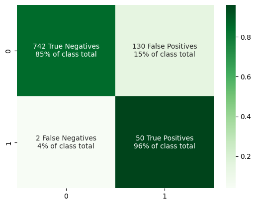
show_confusion(y_test, best_baseline_model.predict(X_test))

We’re already in a really good spot as we are correctly identifying the positive class over 96% of the time. We have more false positives than I’d like, but maybe some hyperparameter tuning can help here.
Step 3: Finding Best Hyperparams with GridsearchCV
For finding the best logistic regression hyperparams, we will use Scikit-Learn’s GridSearchCV in combination with an Imblearn Pipeline. GridsearchCV performs an exhaustive search over the provided parameters and performs cross-validation for every parameter combination. Imblearn’s Pipeline allows us to perform the same resampling technique we chose in step two with GridsearchCV. The pipeline will resample the training data using cluster undersampling but will not touch the balance of the test data in the fold. We’ll set up GridsearchCV to optimize for recall score and have it return the model that performed the best in terms of average recall across all folds.
from imblearn.pipeline import Pipeline
from sklearn.model_selection import GridSearchCV

model = Pipeline([
        # Perform resampling on train split
        ('sampling', ClusterCentroids(estimator=MiniBatchKMeans(n_init=1, random_state=0), random_state=42)),
        ('classification', LogisticRegression(random_state = 42))
    ])

parameters = {'classification__solver':('liblinear', 'lbfgs'), 'classification__C':[1, 5, 10]}

# Returns best model in terms of recall score
best_grid_model = GridSearchCV(model, param_grid = parameters, cv = 5, refit = True, scoring = 'recall')
best_grid_model.fit(X_train, y_train)

# A look at how well all hyperparameter combinations perform
pd.DataFrame(best_grid_model.cv_results_).sort_values(by = 'rank_test_score')
| mean_fit_time | std_fit_time | mean_score_time | std_score_time | param_classification__C | param_classification__solver | params | split0_test_score | split1_test_score | split2_test_score | split3_test_score | split4_test_score | mean_test_score | std_test_score | rank_test_score | |
|---|---|---|---|---|---|---|---|---|---|---|---|---|---|---|---|
| 2 | 29.715823 | 3.306074 | 0.068921 | 0.016334 | 5 | liblinear | {'classification__C': 5, 'classification__solv... | 0.908257 | 0.935780 | 0.936364 | 0.909091 | 0.889908 | 0.915880 | 0.017857 | 1 |
| 3 | 29.644415 | 3.598677 | 0.095378 | 0.026857 | 5 | lbfgs | {'classification__C': 5, 'classification__solv... | 0.908257 | 0.935780 | 0.936364 | 0.909091 | 0.889908 | 0.915880 | 0.017857 | 1 |
| 0 | 29.187842 | 2.767306 | 0.057547 | 0.019141 | 1 | liblinear | {'classification__C': 1, 'classification__solv... | 0.899083 | 0.935780 | 0.927273 | 0.900000 | 0.889908 | 0.910409 | 0.017804 | 3 |
| 1 | 28.689645 | 3.572646 | 0.104958 | 0.027626 | 1 | lbfgs | {'classification__C': 1, 'classification__solv... | 0.899083 | 0.935780 | 0.927273 | 0.900000 | 0.889908 | 0.910409 | 0.017804 | 3 |
| 4 | 28.605801 | 2.047266 | 0.052858 | 0.005150 | 10 | liblinear | {'classification__C': 10, 'classification__sol... | 0.908257 | 0.926606 | 0.918182 | 0.890909 | 0.889908 | 0.906772 | 0.014572 | 5 |
| 5 | 32.235926 | 3.819624 | 0.099514 | 0.020922 | 10 | lbfgs | {'classification__C': 10, 'classification__sol... | 0.908257 | 0.926606 | 0.918182 | 0.890909 | 0.889908 | 0.906772 | 0.014572 | 5 |
A look at the confusion matrix following hyperparameter tuning.
show_confusion(y_test, best_grid_model.predict(X_test))
This is a bit better. Our false positive rate has reduced slightly, meaning that this new model is having an easier time differentiating between the two classes than before. In many cases this would suffice, but what if we attempted to let no positive samples slip past our classifier? This is where the fourth step can come in, altering the decision threshold of the model.
Step 4: Altering the Decision Threshold
Altering the decision threshold will allow us to catch more true positive samples by increasing the sensitivity of the model. This increase in sensitivity will come at a cost, however, causing a decrease in the precision of our model. But, that’s ok! We are most concerned with catching the true positives in this data and aren’t nearly as worried about false positives. Below is a look at our model’s precision-recall curve to get a better understanding of the tradeoff between the two measures prior to changing the decision threshold.
from sklearn.metrics import precision_recall_curve

# Get class probability scores
y_scores = best_grid_model.predict_proba(X_test)[:, 1]

# Returns precision-recall pairs for different probability thresholds
p, r, thresholds = precision_recall_curve(y_test, y_scores)

viz_df = pd.DataFrame({'Precision':p, 'Recall':r})
sns.lineplot(data = viz_df, x = "Recall", y = "Precision")

For us to achieve perfect recall, the model’s precision is going to suffer quite a bit. Again, that’s OK because of this project’s main goal to effectively catch positive samples. Let’s iteratively lower the decision threshold until we achieve perfect recall.
def adjusted_classes(y_scores, t):
    # If pred probability is greater than or equal to threshold it is positive
    return [1 if y >= t else 0 for y in y_scores]

# Default sklearn logistic regression threshold
init_threshold = 0.5
pred = adjusted_classes(y_scores, init_threshold)
recall = recall_score(y_test, pred)

# Stops when recall is perfect
while recall != 1.0:
  init_threshold = init_threshold - 0.001
  pred = adjusted_classes(y_scores, init_threshold)
  recall = recall_score(y_test, pred)

print("Maximum Threshold for Perfect Recall:", init_threshold)
show_confusion(y_test, pred)
Maximum Threshold for Perfect Recall: 0.3679999999999999
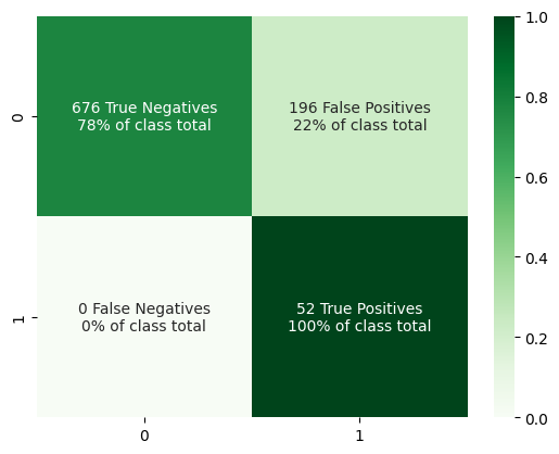
There you have it - a very sensitive model that doesn’t always spit out the positive class!